Example Twitter Analysis
Now that you have collected data from Twitter, what can you do with it? The particulars of any analysis are strongly dictated by the hypotheses being tested. However, many investigations share a common set of objectives early on in their analysis. Solutions to some of these problems are shared below. …
Converting JSON to comma-separated-values (.csv) format
MassMine returns data from all sources as JSON. Depending on your analysis workflow, it can be more desirable to work in a column-oriented data format (such as csv format), such as when importing data into R, Python, SPSS, Excel, or similar. A companion tool has been created called jsan (The JSON Swiss Army k Nife) that provides quick and memory-efficient conversion into column-oriented data formats.
jsan can be used after data has been collected. For example:
# Fetch some data first
massmine --task=twitter-search --count=200 --query=love --output=mydata.json

# Convert the JSON from above into .csv, keeping the
# "text" and "user:screen_name" fields
jsan --input=mydata.json --output=mydata.csv --keep text user:screen_name
Which data fields are available for conversion to csv? This depends on what you have requested from Twitter. If you have collected Twitter data using massmine into a file called “mydata.json”, you can determine which “columns” (i.e., which data fields) are available with jsan using the --list option. The values printed by the following command can be passed to jsan with either the --keep or --remove options.
jsan --input=mydata.json --listFor large data sets, such as when pulling data from the twitter-stream task, it can be advantageous to utilize the streaming capabilities of massmine and jsan to allow conversion while data is being collected:
# Big request, piped into jsan using tee to create a .json file AND a .csv
# copy of the desired fields. This saves the headache of converting a huge
# file later
massmine --task=twitter-stream --query=love --count=2000000 | tee mydata.json | jsan --output=mydata.csv --keep text user:screen_name
To learn more about using jsan, please check the official documentation online.
Loading a massmine dataset into statistical software
To perform any analysis, you must process the data in one of two ways:
- Load the entire dataset into memory
- Read the data file one line at a time
Option 2 is sometimes necessary for extremely large data sets, but requires (arguably) more difficult analysis algorithms designed to operate on streaming, line-by-line data.
Thankfully, memory is cheap and many data sets can safely be loaded into memory all at once. Which option is appropriate depends largely on how much RAM your computer has. The following code snippets share how to accomplish option 1.
Read a CSV dataset into memory in the R Statistical Language
This section assumes you have converted your massmine JSON data into CSV format (see above).
The following snippet assumes your data is in CSV format in a file called “mydata.csv”. Replace the filename when appropriate:
## Read the data into memory. Here we store the results in a
## data frame called tweets
tweets <- read.csv("mydata.csv", header = TRUE, stringsAsFactors = FALSE)

## Data columns can be viewed with the names() function:
names(tweets)

## To extract a given column, use the $ syntax. For example, to extract
## the tweet text for every tweet, use
tweets$text
Read a CSV dataset into memory in Racket Scheme
This section assumes you have converted your massmine JSON data into CSV format (see above).
The following snippet assumes your data is in CSV format in a file called “mydata.csv”. Replace the filename when appropriate:
;;; Required dependency: csv-reading.
;;; Install with `raco pkg install csv-reading`
(require csv-reading)

;;; Read the data into memory. Here we store the results in a
;;; list of lists called tweets
(define tweets (with-input-from-file "mydata.csv"
	 (λ () (csv->list (current-input-port)))))

;;; Data columns can be view by inspecting the first row (i.e., list)
(first tweets)

;;; Assuming the tweet text is the third "column", we index it with 2
;;; (Racket uses zero-indexing). This will return every tweet's text in
;;; your data set
(map (λ (x) (list-ref x 2)) tweets)
“Cleaning” text strings
Often, it is advisable to pre-process, or “clean,” text before beginning any complex analysis. This can take many forms, but often includes:
- Homogenizing character encoding: Some text is represented as ASCII, some as Unicode. Unicode allows for many more characters and is the preferred encoding scheme. Sometimes it is necessary to convert heterogeneous encoding into a common scheme. This is especially true if data from multiple sources will be combined.
- Removing capitalization: When calculating word frequencies, for example, the difference between “home,” “Home,” “HOME,” etc. is uninteresting. Typically, it’s more useful to treat these variations as the same word. This is more easily accomplished by first converting all letters to lowercase.
- Collapsing whitespace: Users often include extra whitespace in their posts, including spaces, tabs, newlines, etc. Typically, these are not meaningful components of the message. Collapsing whitespace usually involves converting sequences of whitespace into single space characters.
- Removing punctuation: Punctuation can be meaningful, such as emoji sequences that convey emotion. Often, punctuation is not meaningful. In these situations, it adds spurious artifacts in an analysis. In these situations, punctuation can be stripped out to leave just the words contained in a message.
Homogenizing character encoding in the R Statistical Language
The following code snippets assume your dataset is loaded into R as a data frame called tweets (see above)
## Convert, as necessary, character encoding to Unicode UTF-8
tweets$text <- iconv(tweets$text, "", "UTF-8")
Removing capitalization in the R Statistical Language
The following code snippets assume your dataset is loaded into R as a data frame called tweets (see above)
## Lowercase everything
tweets$text <- tolower(tweets$text)
Collapsing whitespace in the R Statistical Language
The following code snippets assume your dataset is loaded into R as a data frame called tweets (see above)
## Collapse extra whitespace into single space characters
tweets$text <- gsub("[[:space:]]+", " ", tweets$text)
Removing punctuation in the R Statistical Language
The following code snippets assume your dataset is loaded into R as a data frame called tweets (see above)
## Heavy-handed approach. This removes all punctuation.
tweets$text <- gsub("[[:punct:]]+", " ", tweets$text)
Web links (URLs) are problematic, as they are a mixture of punctuation and characters. If your data contains many URLs, consider removing them BEFORE removing punctuation. Matching URLs is very difficult. The following trick does a decent job of stripping URLs, and then removes punctuation afterward:
## Remove URLs
tweets$text <- gsub("(http|https)([^/]+).*", " ", tweets$text)

## Now remove punctuation
tweets$text <- gsub("[[:punct:]]+", " ", tweets$text)
Identifying hashtags
What #hashtags are present in your data? Let’s find out!
Listing hashtags in the R Statistical Language
The following code snippets assume your dataset is loaded into R as a data frame called tweets (see above)
## What hashtags do we find across all tweets?
hash.regexp <- "#[[:alpha:]][[:alnum:]_]+"
hashtags <- unlist(sapply(1:length(tweets$text), function (x) {
    regmatches(tweets$text[x],
               gregexpr(hash.regexp, tweets$text[x]))}))
The resulting variable hashtags is a vector containing all observed hashtags, including repeats. To determine the frequency of each hashtag in your data set, use the table() function:
## Tabulate the number of occurrences of each hashtag
table(hashtags)

## Better yet, sort frequencies in descending order to see
## which hashtags were the most popular
sort(table(hashtags), decreasing = TRUE)
Identifying @user mentions
What @users are present in your data set? The answer requires a similar strategy to identifying #hashtags
Listing @users in the R Statistical Language
The following code snippets assume your dataset is loaded into R as a data frame called tweets (see above)
## What users do we find across all tweets?
user.regexp <- "@[[:alpha:]][[:alnum:]_]+"
usernames <- unlist(sapply(1:length(tweets$text), function (x) {
    regmatches(tweets$text[x],
               gregexpr(user.regexp, tweets$text[x]))}))
The resulting variable usernames is a vector containing all observed @usernames, including repeats. To determine the frequency of each user in your data set, use the table() function:
## Tabulate the number of occurrences of each @username
table(usernames)

## Better yet, sort frequencies in descending order to see
## which usernames were the most popular
sort(table(usernames), decreasing = TRUE)
Time series: Tweet frequency as a function of time
The following code snippets assume your dataset is loaded into R as a data frame called tweets (see above)
Trending topics can quickly increase and decrease in popularity on Twitter. Visualizing how frequently tweets are occurring can be useful for diagnosing such patterns. In the following example, one can replace the “day” in cut(tweets.date, breaks = "day") with “hour”, “week”, and “month” as appropriate.
## Convert date strings to date data type
tweets.date <- as.POSIXct(tweets$created_at, format = "%a %b %e %T %z %Y")

## Index each tweet by the day of its creation
day.index = cut(tweets.date, breaks = "day")

## Count how many tweets occurred on each day
tmp <- sapply(levels(day.index),
  function(x) length(which(day.index==x)))

## Isolate the tweet frequencies
counts <- as.vector(tmp)

## Plot tweet frequency by day
plot(1:length(counts), counts, type="o", lwd = 2,
     xlab = "Days", ylab = "Frequency",
     main = "Tweet Frequency As A Function Of Days")
grid(col = "darkgray")
The zoo package in R provides additional support for working with time/date information. To use the package, first install it:
install.packages("zoo")After loading the package…
library(zoo)…the final plotting procedure can be improved to include the actual dates on the x-axis:
## Create x-axis increments for each day
days <- as.Date(names(tmp))

## Plot tweet frequency by day
plot(days, counts, type="o", lwd = 2,
     xlab = "Days", ylab = "Frequency",
     main = "Tweet Frequency As A Function Of Days")
grid(col = "darkgray")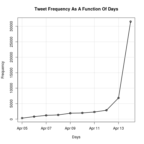
Text Mining Using R’s TM Package
R’s TM package provides many standard text mining functions that are useful for Twitter text analysis. Documentation for the TM package is available here.
The following assumes that you have already read your Twitter data into the tweets variable using the read.csv() example listed above, and that you have already homogenized character encoding, removed capitalization, collapsed whitespace, and removed punctuation.
First, install the TM package:
install.packages("tm")Removing Additional Words from Twitter Text
In addition to the text transformations already completed, it is usually necessary to remove other words for analysis. Stopwords are common words like “the,” “and,” “it,” “there,” and they will confound word frequency analyses if they are not removed. The following will remove English stopwords from text data in TM:
tweets$text <- removeWords(tweets$text, stopwords(kind="en"))Sometimes there are other words that need to be removed for reasons pertaining to a specific project or because of particular research question. First, create a variable containing the list of additional words to be removed:
word.list <- c("cat", "dog", "horse", "chicken")Next, using the same removeWords() function, remove the list of words from the tweets$text vector:
tweets$text <- removeWords(tweets$text, word.list)Creating a Corpus and Document-Term Matrix in TM
A “corpus” is a data type used specifically by the TM package. Using the tweets$text vector that contains the tweet texts from the “love” data collection, we can transform this collection of “documents” into a corpus with the following function:
corpus <- VCorpus(VectorSource(tweets$text))Once the tweet texts are changed to TM’s corpus data type, it can be easily analyzed as a document-term matrix:
dtm <- DocumentTermMatrix(corpus)Summary Statistics of Tweet Texts
By entering just the document-term matrix variable into the REPL, TM will return summary statistics for the corpus: the number of documents (tweets), the number of original words, sparsity, maximal word length, and weighting.
dtmRemoving Sparse Words
The removeSparseTerms() function in the TM package will remove sparse (infrequently occurring) words from the corpus of tweet texts. Based on the summary statistics provided in the previous example, we can use the “sparsity” percentage to determine how many sparse terms to remove. The 0.1 argument in the function below determines what percentage of sparse terms to remove. It is a good idea to save the new document-term matrix with sparse words removed in a different variable in case your first attempt removes too many words:
dtm1 <- removeSparseTerms(dtm, 0.1)Word Frequencies
Word frequency totals can be returned as a vector by summing the columns of terms in the matrix:
freq <- colSums(as.matrix(dtm1))Using the head() and table() functions, we can see the top 20 most frequent terms in the corpus:
head(table(freq), 20)Word Correlations
Word correlations can be determined with the findAssocs() function in the TM package. The function below finds which terms are most associated with the word “love” and returns a vector of decimal percentages. If the returned value is 1.0 for a particular word, then has a correlation coefficient of 1 in relationship to the word “love” in a given corpus. The corlimit argument allows users to determine a correlation threshold. So, if the corlimit argument is set to .5, then any words with a correlation coefficient of less than that will be ignored. For exploratory analyses, reducing the corlimit to 0.0 will return all correlations with a particular term, but for research purposes a minimum of .5 is recommended (and depending on the research question or the claims made about particular associations 0.8 or higher may be necessary). Using the word.co variable to save the returned vector, the following function determines word co-occurrence:
word.co <- findAssocs(dtm, "love", corlimit=0.0)Using the head() function again, we can see the top 20 words that co-occur with “love” in the tweet texts:
head(word.co, 20)Be careful when using word correlation analyses with Twitter data over very short periods of time. High volumes of retweets by users can create many 100% correlation values. Retweets are designated with RT appearing at the beginning of a tweet’s text, and it may be necessary for you to remove all retweeted tweets from your corpus. However, if your dataset has been collected over a long enough period of time (this is a relative determination based on the activity of a particular trend or dataset), then retweets should not cause a problem.
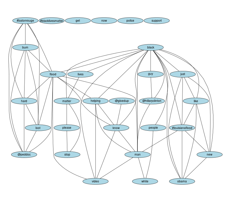
Word Association Graph
The following data visualization is created using the Rgraphviz package and the TM package in R. The rationale for this visual is taken from the initial publication about TM in the Journal of Statistical Software. This cluster graph is useful for visualizing associations among the most frequent terms in a corpus of Tweets, and if # and @ symbols are retained after cleaning a corpus, then it provides a visual for how the top terms in a corpus are associated with the top hashtags and username mentions. Using the data on the top word frequencies in the corpus, as shown above, the following code plots the associations among the top 30 words in a corpus:
# Reduces the list of the most frequent terms to the top 30
freq <- head(sort(freq, decreasing=TRUE), 30)

# Turn the frequency data type returned from TM (double) into an R data frame
freq <- data.frame(names(freq), as.numeric(freq))

# Rename the columns according to their contents
colnames(freq) <- c("Word", "Freq")

# Sets the low frequency threshold equal to the 30th term
lowNum <- tail(freq$Freq, 1)

# Sets the high frequency threshold equal to the top term
highNum <- head(freq$Freq, 1)

# The png() device saves the plot as an image to the working directory
png("corGraph.png", 800, 700)

# Calls additional attributions for changing the color and shape of nodes
defAttrs <- getDefaultAttrs()

# Creates the cluster graph. To change the correlation threshold for drawing
# the edges in the graph, adjust the correlation coefficient provided to the
# corThreashold argument
plot(dtm, terms=findFreqTerms(dtm, lowfreq=lowNum, highfreq=highNum),
     corThreshold=0.1, attrs=list(node=list(shape = "ellipse", fixedsize = FALSE,
                                            fillcolor="lightblue", height="2.6", width="10.5",
                                            fontsize="14")))

# Saves the graph to file and closes the png() device
dev.off()
Using the above code, the following graph was created using data collected from Twitter’s Rest API with the query “blacklivesmatter”: